Deep Cleaning: It's a real bear!
Managing data for a deep learning project can be a real bear. For one thing, the datasets tend to be large (as in big data). In addition to your dataset, you may also be generating a lot of intermediate data and large neural network weight files. For any deep learning project you need to consider things like storage, organization, labeling and cleaning the dataset. This can be a very time consuming (and not so glamorous) aspect of deep learning projects!
For the BearID Project, we’re currently following an approach based on FaceNet. Their dataset included hundreds of millions of images of millions of different individuals. Our dataset isn’t nearly as large as that, but it’s still many thousands of images. This article examines our approach to managing the data.
Storing Large Datasets
Deep learning is generally synonymous with large datasets. Our current dataset is about 80GB, though we expect it to grow by as much as an order of magnitude (and that’s still not large in comparison). During the training process, we may create a lot of new data, such as intermediate images, metadata and network weights files. All this data can add up.
Speed is another consideration. You most likely won’t be able to load all of your data into memory at one time (especially when using GPU acceleration), so you’ll have to load batches of data at a time. You want to be able to load the data as quickly as possible. You can hide some of the loading time by having your CPU start processing the next batch while your GPU is training the current batch, but fast storage can still be beneficial.
We built our deep learning computer with a fairly fast (up to 540 MB/s for reads) Solid State Drive (SSD). They are more expensive than traditional Hard Disk Drives (HDD), so we only got a 500GB SSD. As our dataset grew (and as we started working with other datasets, like for Kaggle competitions), we decided to add a 4TB HDD which runs at about 1/3 the speed of the SSD (up to 180 MB/s). We can store all our datasets on the HDD and copy over working sets to the SSD as needed.
Just to be safe, we also back up our key datasets on a portable drive and a Network Attached Storage (NAS) system.
Organizing the Data
How you organize your data is somewhat dependent on your application. For a basic image classification problem, you probably have a bunch of images and a set of metadata containing the labels for the images. You split your data into training and test data, pick some architectures and have at it.
The bearid application reads in a photo and outputs a bear ID, much like a typical image classifier. However, as described in previous posts (FaceNet for Bears), the BearID application follows a four stage pipeline:
- Find the face (
bearface) - Reorient each face (
bearchip) - Encode the face (
bearembed) - Match the face (
bearsvm)
Each stage, aside from bearchip, incorporates a neural network that requires training. Each stage has a set of inputs and outputs that need to be organized. The basic flow is as follows:
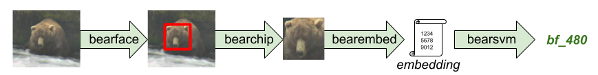
bearface- Takes a source image and outputs a bounding box and 5 face points (eyes, ears and nose) for each bear face. It writes out this metadata in an XML file. It uses a neural network from dlib which was trained on dog faces. As we grow our bear dataset, we will retrain the network on bears.bearchip- Take a source image and metadata and writes out a face chip (pose normalized, cropped image). We will need to experiment with the parameters for normalization and cropping.bearembed- Takes a face chip and outputs an embedding file. It uses a neural network which was trained using our initial data. We will need to retrain using different datasets as well as different parameters forbearfaceandbearchip.bearsvm- Takes an embedding file and determines the ID of the bear using a Support Vector Machine (SVM). The SVM will be retrained as the embeddings change. We may also choose to replace it with a different classifier method.
During training, each stage utilizes large sets of input data and generates large sets of output data. We will likely run many experiments with each stage. We need to manage the results of all the experiments.
Source Data
Our source data consists of photos of bears. The photos come from a number of different contributors (park staff, researchers, photographers, etc.) taken a different locations (Brooks Falls, Glendale Cove, etc.). We decided to keep our contributors separated so we can more easily trace back to the source and discern new data from older data. Since bears also change in appearance over the years (and even over the course of one year), we wanted to keep some date information.
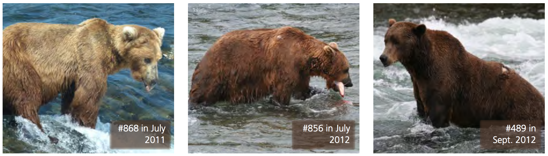 Image courtesy of Katmai National Park
For simplicity, we decided to use a directory structure rather than implement a database. We have a top level directory with sub-directories for each location. Under each location, we have directories for each contributor and date of contribution. Under each contributor, we have a directory for each bear in the dataset and separate directories for photos containing unknown bears and/or multiple bears (including cubs). Our directory structure looks something like this:
image_source/
├── location_01
│   └── contributor01_date
│       ├── bear_id_01
│       ├── ...
└── location_02
    ├── contributor02_date
    │   ├── bear_id_01
    │   ├── ...
    │   ├── bear_unknown
    │   └── bear_multiple
    └── contributor03_date
        ├── bear_id_cub
        └── ...
When we receive photos from contributors, they are not necessarily structured the same way. We move them around manually or with scripts. The bear_id directory names are unique identifiers per location which serve as the labels (more on labeling later). We generate XML files to collect the various images into the training, validation and test sets we want to utilize.
Result Data
As we experiment with each stage, we keep the results to be used for subsequent stages. Since each stage of the pipeline depends on the previous stage, we decided to structure our results accordingly:
face_config_01
├── face_meta
├── chip_config_01
│   ├── chip_meta
│   ├── chip_images
│   │   ├── location_01
│   │   │   ├── bear_id_01
│   │   │   └── ...
│   │   └── location_02
│   │       └── ...
│   ├── embed_config_01
│   │   ├── embed_meta
│   │   ├── embeddings
│   │   │   ├── bear_id_01
│   │   │   └── ...
│   │   ├── class_config_01
│   │   │   ├── class_meta
│   │   │   └── classifier_01
│   │   ├── class_config_02
│   │   |   └── ...
│   │   └── ...
│   ├── embed_config_02
│   │   └── ...
│   └── ...
├── chip_config_02
│   └── ...
└── ...
face_config_02
└── ...
face_config_XX: The top levels correlate to thebearfacestage. Each bear face configuration has a separate directory for its results (face_config_01,face_config_02, …). Results include the face metadata XML files (bounding box, face points and ID labels) and thebearfaceneural network configuration and weights. Currently we have only 1 face configuration based on manually adjusted labels (more on labels below). This will change when we retrain thebearfacenetwork.chip_config_XX: The second levels correlate to thebearchipstage. Since the inputs are different for eachbearfaceconfiguration, they appear under the appropriateface_config_XX. Eachbearchipconfiguration will produce different results, so there are multiplechip_config_XXunder eachface_config_XX. The results include the face chip images and relevant metadata.embed_config_XX: The third levels correlate to thebearembedstage. Again they appear under eachchip_config_XX. Training the embedding network with different chip configurations and different parameters will result in new network weights. For a given set of parameters and weights, a full set of embeddings is generated.class_config_XX: The final levels correlate to thebearsvmstage. They appear under eachembed_config_XX. While we are currently using an SVM for classification, this is something we will experiment with. Training the classifier with new embeddings and architectures will result in different networks and weights. These are the final outputs of the training process.
As we try different experiments, some will be successful, and some not. We can abandon the unsuccessful paths and focus on those which are more promising. Our path from source image to bear ID with the best results (based on our metrics) will be used for the end-to-end bearid application.
Labeling the Data
Labeled training data is the cornerstone of supervised learning. In our case, the main labels we deal with are the bear identity and the face metadata.
Bear Identities
Each source image is labeled with the ID of the bear(s) in the image. The labels are given by experts in the field who (hopefully) really know the bears. Generally contributors provide us photos which have been sorted into directories with the ID of the bear. Occasionally the bear ID is part of the file name. In either case, we copy them into the directory structure described previously. We carry the labels through all the metadata that we generate along the way so it can be utilized by the appropriate training and testing code. The bear ID is utilized by both bearembed and bearsvm.
| ID | Example Face Images |
|---|---|
| Also | 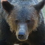 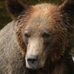 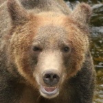 |
| Beatrice | 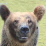 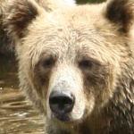 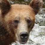 |
| Chestnut | 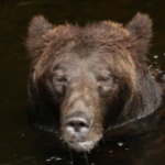 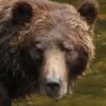 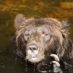 |
Images courtesy of the Brown Bear Research Network
Face Metadata
The face metadata to train bearface is more cumbersome. To create a face and key point detector, you need to label each source image with a bounding box for the face and point for each of nose, left eye, right eye, left ear and right ear.
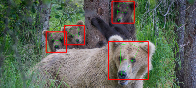 Image Courtesy of Katmai National Park
Fortunately, we were able to use an example program from the Dlib Toolkit called Dog Hipsterizer (see the post Hipster Bears). It works pretty well with bears, but not perfectly. We run all our source images through a modified version of the dog hipsterizer to get the initial face metadata XML files. Then we use another dlib tool called imglab to manually fix the boxes and key points. As our dataset grows, maybe we can farm this task out to volunteers or to a platform like Amazon Mechanical Turk.
Cleaning the Data
The final point I’ll cover here is data cleaning. Essentially, you want the dataset to represent the problems you are trying to solve as accurately as possible. After all: garbage in; garbage out.
- Unwanted observations: Duplicate and irrelevant observations (such as images with no bears) should be removed.
- Structural errors: The images should be in a supported format. The labels should follow the same formats in our directory structure and XML files.
- Unwanted outliers: Remove really poor quality images. Separate out cubs because they change so dramatically. We are also examining how the pose of the bear affects our results and may need to remove images with extreme poses (see example poses below).
- Missing values: Make sure all the data have the necessary labels.
- Imbalanced classes: For some bears we have a small number of images (or no images). We may leave them out of the training and test sets and reserve them as a hold out set. We can use these images to test how well the end to end system handles unknown bears.
Here are some examples which illustrate how the pose of a bear can impact the face chip, even when normalized:
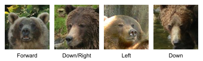
Images courtesy of the Brown Bear Research Network
Conclusion
Managing data for a deep learning can be a chore. At the outset you should consider issues like storage, organization, labeling and cleaning. If you address each of these issues well, you will have higher productivity, improved performance and better results. It’s always a good time for spring cleaning!