BearID 1.0
In the last post, Bear (C)hipsterizer, we talked about using a Dlib Toolkit example program, Dog Hipsterizer, to find bear faces and face landmarks. The example program used a CNN based face detector trained for dogs, mmod_dog_hipsterizer.dat, which happened to work for bears as well. We used the face detections and landmarks from the network to reorient, align and crop the bear face. We then wrote out a 150x150 pixel face chip for each bear face. At that point, we had completed the first two stages of our bear ID pipeline: stage 1 (Find the Face) and stage 2 (Reorient Each Face). We made a program called bearchip, which takes a set of input images and outputs the oriented face chips. We execute it like this:
./bearchip mmod_dog_hipsterizer.dat <image_dir>
That left us with two more stages: stage 3 (Encode the Face) and stage 4 (Match the Face).
Encode the Face
The purpose of this stage is to train a neural network to to generate a 128-dimensional vector, an embedding, for a given 150x150 pixel face chip. The training process utilizes pairs of chips and learns to make the embeddings for chips of the same bear to be “close” in 128-D space, and make the embeddings for chips of different bears to be “far” in 128-D space. Once you have trained the network, you can generate embeddings for each bear face chip. State of the art networks for human face embedding are able to predict if two faces are the same person with greater than 99% accuracy. The embeddings can be used with your favorite classifying, clustering or other machine learning algorithms.
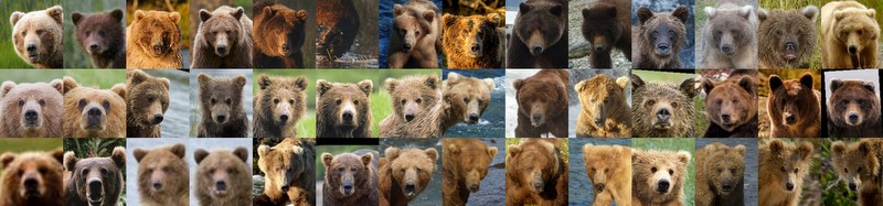
Once again, dlib has a great example, which is described in High Quality Face Recognition with Deep Metric Learning. We started with a set of more than 1000 images made up of 28 individual brown bears from the Brooks Falls area. We used the bearchip program to find bears and generate face chips. We manually filtered out “bad” chips, and ended up with a set of about about 800. We split the data into a training set and a test set. Following the dlib example, we trained an embedding network on the training set.
Our embedding program, bearembed, takes a directory, face_chip_dir, which has subdirectories for each individual bear. The subdirectories contain face chips for that bear. We can train the embedding network using a command like this (where face_chip_dir is the directory containing the training set):
./bearembed -train <face_chip_dir>
We can validate the network using the test data with this command:
./bearembed -test <face_chip_dir>
The resulting network is able to predict if any two faces from the test set are of the same bear with around 90% accuracy. The accuracy on the training set was 100%, which means we most likely overfit the network. We’ll need to deal with that later by increasing the size of our dataset.
Finally, we can generate embeddings for every bear face chip with this command (where face_chip_dir is a directory containing all the bears we want to embed and embed_dir is the directory where the embeddings are stored):
./bearembed -embed <embedded_dir> <face_chip_dir>
The embedding data is written out using dlib’s serialize function. The directory structure follows the structure of the face chip directory.
Match the Face
This is supposed to be the easiest step in the whole process. We simply need to find the bear in our dataset with the closest match to the embedding. This is typically done with a basic machine learning classifier, such as a Support Vector Machine (SVM). It fact, this step is not very hard, but it was the first step where we didn’t have an explicit example to follow. There are a few examples of SVM classifiers in dlib, so we used a mash up of those, plus the classifier.py demo from OpenFace.
Using dlib’s SVM routines, we made a multiclass SVM classifier using a linear kernel and one-vs-one (OvO) reduction methodology. Our program, bearsvm, reads in all the embeddings to create a set of samples and labels, then trains the OvO SVM classifier. The program runs cross-validation (although we did not yet separate the embeddings into training and test data) and saves the trained SVM. We execute the program like so:
./bearsvm <embedded_dir>
We tried a few different values of the soft margin parameter C, running a 5 fold cross-validation on each. We stuck with one that gave us pretty good results. We can fine tune this and try other classifiers later.
Putting It All Together
Once we created and trained all four stages in our pipeline, we needed to put it all together to create the actual bear identifier, bearid. The goal of this program is to read in an image, find any bears in the image and identify them. This program executes the complete pipeline:
- Find the Face: Read in the image and apply the face detection network (from the dog hipsterizer) to find each bear.
- Reorient Each Face: For each detected face, use the detected landmarks to reorient, scale and crop the face to make a face chip.
- Encode the Face: Run each face chip through the embedding network we trained with
bearembedto generate a 128-D face embedding. - Match the Face: Run each face embedding through the OvO SVM we trained in
bearsvmto get an identification.
We run the program like this:
./bearid <image_file>
It works! Well, mostly. All the pieces are working, but as you can imagine they each introduce some amount of error. The bearid program does a pretty good job at identifying the bears in the images we have in our training and test sets, so we excitedly downloaded some additional images of bears from Brooks Falls. The results using the never before seen images were less than stellar. This isn’t too surprising. The state of the are human face recognition networks are trained with millions of faces. We only used about 800.
Next Steps
We have completed version 1.0 of our BearID program. The main thing we need to do to improve the accuracy is to get more data to retrain the various stages of our pipeline (especially the embedding network). We are attempting to get photos directly from the National Park Staff as well as finding more galleries from visitors to Brooks Falls. We can look at other populations of brown bears with well known individuals (including captive bears). We can also try to use videos of the bears to extract images.
In addition to growing our dataset, we need analyze the accuracy of each stage of the pipeline and calculate better metrics to compare strategies. Here are some things we know we can do to improve each stage (although we need the metrics to quantify any improvements):
- Stage 1: Train our own face and landmark detector, rather than using the dog hipsterizer network. This will require not only a lot more data, but also a lot of manual labeling.
- Stage 2: Try to improve our face alignment and/or filter out faces which don’t align well.
- Stage 3: Train with a lot more face chips (and make sure the chips are well aligned)!
- Stage 4: Fine tune our SVM or consider using a different methodology.
We will explore all of these ideas, as well as new ideas, as we continue to expand our dataset. Check back here to see our progress.