Too Good To Be True

This week Dr. Melanie Clapham is presenting the BearID Project at the International Conference on Bear Research & Management in Slovenia. In the abstract for the presentation, titled “Developing Automated Face Recognition Technology for Noninvasive Monitoring of Brown Bears (Ursus Arctos)” (abstract ID 237 in the conference book of abstracts), we list a preliminary accuracy of 93.28 ± 4.9% for our face embedding network, bearembed. Considering that state of the art human face recognition is well above 99.5% on the Labeled Faces in the Wild (LFW) test set, our number seemed plausible. However, as we were updating our findings for the presentation, we found our story to be quite different.

Face Embedding from dlib

As stated in previous posts, the BearID Project follows an approach based on FaceNet and utilizes networks and examples from dlib. For bearembed, we use a network for human face detection implemented in dlib (see this blog post). The example program, dnn_face_recognition_ex.cpp, implements a clustering algorithm using a pre-trained embedding network for human faces. To train the network on bears, we followed another example program, dnn_metric_learning_on_images_ex.cpp.

Testing Face Embedding

The premise is to take 2 face images and generate embeddings (run each face image through the bearembed network). Calculate the distance between the embedding results and compare. If the distance is less than a specified threshold, then the bears are the same. If the distance is greater than the threshold, then they bears are different.

The dlib example has a very rudimentary test set up. It builds a batch of data by randomly selecting M IDs and randomly selecting N face images for each ID. The values of M and N were both 5. So for one test batch, we would get 5 faces from 5 different bears. Generating all the combinations of 2 from the 25 faces results in 50 matching pairs (both faces are of the same bear) and 250 non-matching pairs (both images are of different bears). We decided to run through 100 batches (or folds), then average the results. We were getting and average accuracy of 93.28.

Problems with the Test Procedure

To compare an application’s ability to discriminate between pairs of faces, many researchers use the Labeled Faces in the Wild (LFW) data set. The LFW data set contains more than 13,000 images of faces collected from the web. For testing, the data set is split into 10 folds. Each fold contains 300 matching pairs and 300 non-matching pairs. Once you have a candidate network (which may be trained with outside data depending on your entry category), you generate test results by using a cross-validation. Essentially, use 9 folds for training and 1 fold for testing. Do this 10 times, using a different fold for testing each time, then average the results. If you are training with outside data, simply test against each fold of the LFW data set and average the result.

Problem 1: Unbalanced Test Data

In our test set up, we were using 50 matching pairs and 250 non-matching pairs. This ratio of 1 matching to 5 non-matching pairs skews the results giving more weight to the network’s ability to determine if bears are different and less weight to the network’s ability to determine if bears are the same. Our metric, accuracy, is the number of correct prediction over the total number of tests. You can split this into two parts by looking at the networks accuracy on positive cases (True Positive Rate, or TPR) and negative cases (True Negative Rate, or TNR). Multiplying the TPR and TNR by the ratio of positive/negative examples and adding together yields the accuracy:

Accuracy = TPR * Positive Ratio + NPR * Negative Ratio

From our previous results, our network had a TNR of ~98% and a TPR of ~65%. So the network is predicting negative examples much better than positive examples. Since our test set has more negative examples (250/300) than positive examples (50/300), our accuracy was skewed higher:

Accuracy = (65 * 50/300) + (98 * 250/300) ~= 93%

If we use an even ratio of positive examples and negative examples we should get a lower accuracy:

Accuracy = 65 * 0.5 + 98 * 0.5 = 81.5%

Problem 2: Repeated Images

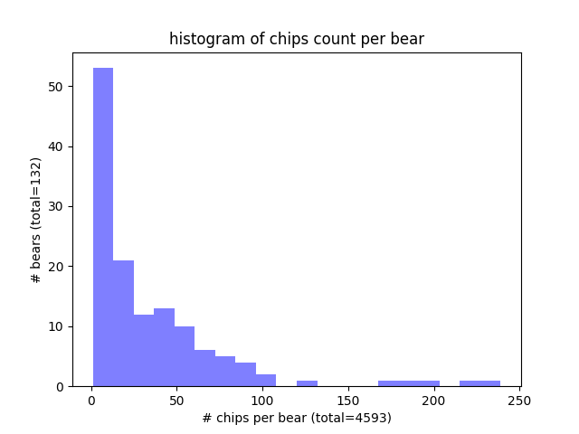
The second problem with the test set up we used is related to the number of face images (chips) we have per bear. In the histogram above you can see that we have a few bears (>50) with few face chips (<10). In our test set, which is 20% of the data, most of the bears have less 5 chips. Our test set up will still randomly pick those labels, and will pick 5 faces, even when there are not five, by picking the same face more than once. If there’s only one face, it will use that face 5 times. The embedding of a given face is deterministic. So if we compare a face to itself, it will always match. This skewed our TRP to be higher than it should be. If we guarantee a face chip is not compared to itself, the TPR goes down to ~45% while the TNR remains about the same. This leads to an even lower accuracy:

Accuracy = 45 * 0.5 + 98 * 0.5 = 72%

New Test Procedure

Our new test procedure more closely resembles LFW. We split the test set into folds and make sure of the following:

• Each fold has an even number of positive and negative examples.
• A given face image is never compared with itself.
• All of the pairs in our test set are unique (positives and negatives).

As expected our reported accuracy went down to the low 70’s. Fortunately we have already made some improvements in the training process and have some other ideas in mind. We’ll explore those in later posts, so stay tuned!